7.2 Measures of Dispersion (Introduction)
(A) Determine the range of a set of data
1. For an ungrouped data,
Range = largest value – smallest value.
2. For a grouped data,
Range = midpoint of the last class – midpoint of the first class.
Example 1:
Determine the range of the following data.
(a) 720, 840, 610, 980, 900
(b)
Time (minutes) |
1 – 6 |
7 – 12 |
13 – 18 |
19 – 24 |
25 – 30 |
Frequency |
3 |
5 |
9 |
4 |
4 |
Solution:
(a)
Largest value of the data = 980
Smallest value of data = 610
Range = 980 – 610 = 370
(b)
Midpoint of the last class
= ½ (25 + 30) minutes
= 27.5 minute
Midpoint of the first class
= ½ (1 + 6) minutes
= 3.5 minute
Range = (27.5 – 3.5) minute = 24 minutes
(B) Medians and Quartiles
1. The first quartile (Q1)is a number such that 1 4 of the total number of data that has a value less than the number.
2. The median is the second quartile which is the value that lies at the centre of the data.
3. The third quartile (Q3) is a number such that 3 4of the total number of data that has a value less than the number.
4. The interquartile range is the difference between the third quartile and the first quartile.
Interquartile range = third quartile – first quartile |
Example 2:
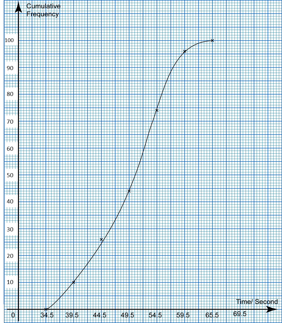
The ogive in the diagram shows the distribution of time (to the nearest second) taken by 100 students in a swimming competition. From the ogive, determine
(a) the median,
(b) the first quartile,
(c) the third quartile
(d) the interquartile range of the time taken.
Solution:
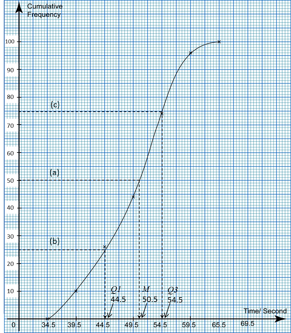
(a)12of 100 students=12×100=50From the ogive, median,M=50.5second(b)14of 100 students=14×100=25From the ogive, first quartile,Q1=44.5second(c)34of 100 students=34×100=75From the ogive, third quartile,Q3= 54.5second
(d)
Interquartile range
= Third quartile – First quartile
= 54.5 – 44.5
= 10.0 second